Elementary quantum computing

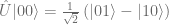
For theoretical physicists, programming quantum computers sounds like one of the easiest things to do. It is just playing with tensor products of two-dimensional Hilbert spaces and constructing certain unitary operators. However, we are not such common species and some other people would also like to learn a bit more about quantum computing as well. Therefore, here I will show what the basics of quantum computing are. My approach is to present a very simple example of how to construct a quantum circuit and execute it on a real quantum computer. Namely, we will use publicly available IMB Q Experience platform to generate one of the so-called Bell states:

$| B \rangle = \frac{1}{\sqrt{2}} \left(|01\rangle -|10\rangle \right)$ .

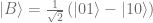
This state has quite interesting physical interpretation. It represents maximally entangled state of two spin 1/2 particles (e.g. two electrons) such that the total spin of the system is equal zero (such states are known as singlets). The $| B \rangle$ state is relevant in both quantum computing and quantum cryptography. So, let us begin…

howtomeasure — Picture of the IBM quantum chip composed of 7 superconducting qubits. Source

A single qubit is a state (vector) $| \Psi \rangle$ in two-dimensional Hilbert space, which we denote as $\mathcal{H}$ . Let us choose the space to be spanned by two orthonormal basis states $|0\rangle$ and $|1\rangle$ such that $\langle 1|0\rangle =0$ and $\langle 0|0\rangle = 1 = \langle 1|1\rangle$ . A general qubit is a superposition of the basis states:

$| \Psi \rangle = \alpha|0\rangle +\beta |1\rangle$ ,

where, $\alpha, \beta \in \mathbb{C}$ (complex numbers), and the normalization condition $\langle \Psi | \Psi \rangle = 1$ implies that $|\alpha|^2+|\beta|^2=1$ .

There are different quantum operators (gates) which may act on the quantum state $| \Psi \rangle$ . For instance, the so-called bit-flip operator $\hat{X}$ which transforms $|0\rangle$ into $|1\rangle$ and $|1\rangle$ into $|0\rangle$ ( $\hat{X}|0\rangle =|1\rangle$ and $\hat{X}|1\rangle =|0\rangle$ ) can be introduced. Another important operator is the Hadamard operator $\hat{H}$ which is defined by the following action on the qubit basis states:

$\hat{H}|0\rangle =\frac{1}{\sqrt{2}}\left(|0\rangle +|1\rangle\right)$ and $\hat{H}|1\rangle =\frac{1}{\sqrt{2}}\left(|0\rangle -|1\rangle\right)$ .

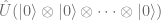
The above are examples of operators acting on a single qubit. However, while considering quantum computing we usually deal with quantum register composed of $N$ qubits. The resulting quantum state belongs to Hilbert space being a tensor product of $N$ copies of the qubit Hilbert space:

$\underbrace{\mathcal{H}\otimes\mathcal{H}\otimes \dots \otimes\mathcal{H}}_{N}$ ,

dimension of which is

$\text{dim}(\underbrace{\mathcal{H}\otimes\mathcal{H}\otimes \dots \otimes\mathcal{H}}_{N})=2^N$ .

This exponential growth with $N$ is the main obstacle behind simulating quantum systems on classical computers. With the present most powerful classical supercomputers we can simulate quantum systems with ${\bf N=56}$ at most. The difficulty is due to the fact that quantum operators acting on $2^N$ dimensional Hilbert space are represented by $2^N\times2^N$ matrices, which are very difficult to deal with when $N$ is roughly more than $50$ (for $N=56$ , $2^{56} \sim 10^{17}$ ).

A quantum algorithm is simply a unitary operator $\hat{U}$ acting on the initial state of $N$ quibits $|0\rangle\otimes|0\rangle \otimes \dots \otimes|0\rangle \in\mathcal{H}\otimes\mathcal{H}\otimes \dots \otimes\mathcal{H}$ . The outcome of the quantum algorithm is obtained by performing measurements on the final sate: $\hat{U}(|0\rangle\otimes|0\rangle \otimes \dots \otimes|0\rangle)$ . Because of the probabilistic nature of quantum mechanics, the procedure has to be performed repeatedly in order to reconstruct the final state.

The unitary operator $\hat{U}$ can be decomposed into elementary operators called quantum gates, similarly to the logical electronic circuits which are built out of elementary logic gates. The already introduced $\hat{X}$ and $\hat{H}$ operators are examples of gates acting on a single qubit. However, the gates may also act on two or more qubits. An example of 2-qubit gate relevant for our purpose is the so-called CNOT gate, which we denote as $\hat{C}$ . The operator is acting on 2-qubit state $|ab\rangle \equiv |a\rangle \otimes|b\rangle$ , where $|a\rangle$ and $|b \rangle$ are single quibit states. Action of the CNOT operator on the basis states can be expressed as follows:

$\hat{C}(|a\rangle \otimes|b\rangle) =|a\rangle \otimes|a\oplus b\rangle$ ,

where $a,b \in \{0,1\}$ . The $\oplus$ is the XOR (exclusive or) logical operation (or equivalently addition modulo 2), defined as $0\oplus 0 = 0$ , $0\oplus 1 = 1$ , $1\oplus 0 = 1$ and $1\oplus 1 = 0$ . In consequence:

$\hat{C}|00\rangle =|00\rangle$ , $\hat{C}|01\rangle =|01\rangle$ , $\hat{C}|10\rangle =|11\rangle$ , $\hat{C}|11\rangle =|10\rangle$ .

We are now equipped to address the initial task of creating the Bell state $| B \rangle = \frac{1}{\sqrt{2}} \left(|01\rangle -|10\rangle \right)$ . We will perform it in the following steps:

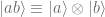
We begin with the initial 2-qubit state $|00\rangle \equiv |0\rangle\otimes|0\rangle$ .
Then, we are acting on both qubits with the spin-flip operator $\hat{X}$ . The corresponding operator has a form of the following tensor product: $\hat{X}\otimes \hat{X}$ . Action of this operator on the initial state gives: $(\hat{X}\otimes \hat{X})(|0\rangle\otimes|0\rangle ) =(\hat{X}|0\rangle\otimes\hat{X}|0\rangle)=|1\rangle\otimes|1\rangle \equiv |11\rangle$ .
Now, let us act on the first quibit with the Hadamard operator (gate), leaving the second qubit unchanged. Such operation is represented by the operator $\hat{H}\otimes\hat{I}$ , where $\hat{I}$ is the identity operator which does not change a quantum state. Action of $\hat{H}\otimes\hat{I}$ on $|11\rangle$ gives $\frac{1}{\sqrt{2}}(|0\rangle -|1\rangle)\otimes |1 \rangle = \frac{1}{\sqrt{2}}|01\rangle-\frac{1}{\sqrt{2}}|11\rangle$ .
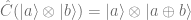
In the final step we are acting on the obtained state with the CNOT gate: $\hat{C}(\frac{1}{\sqrt{2}}|01\rangle-\frac{1}{\sqrt{2}}|11\rangle )=\frac{1}{\sqrt{2}}\hat{C}|01\rangle-\frac{1}{\sqrt{2}}\hat{C}|11\rangle =\frac{1}{\sqrt{2}} \left(|01\rangle -|10\rangle \right)$ , getting the Bell state.

The total unitary operator representing our quantum algorithm can be written as a composition of the elementary steps:

$\hat{U} =\hat{C}(\hat{H} \otimes \hat{I} )(\hat{X} \otimes \hat{X})$ .

Action of this operator on the initial state $|00\rangle$ gives the state $| B \rangle$ :

$\hat{U}|00\rangle =\frac{1}{\sqrt{2}} \left(|01\rangle -|10\rangle \right)$ .

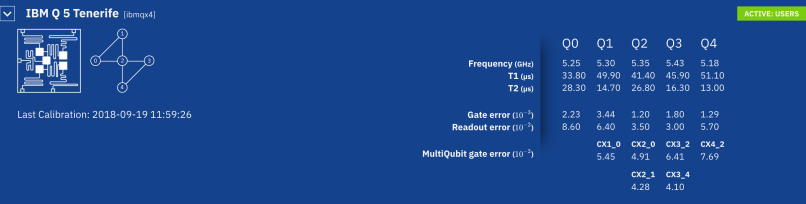
In the experimental part we will create the Bell state employing publicly accessible 5-qubit quantum computer provided by IBM. In the quantum device, qubits are constructed using superconducting circuits, operating at millikelvin temperatures. Access to the device can be obtained through this link (you have to create a free account and login).

IBMQ5

The quantum circuit representing the operator $\hat{U}$ can now be created using the quantum gates in the online quantum composer. The quantum circuit should look as follows (we used the last two qubits here):

Algorithm

The green boxes with letter $X$ represent the bit-flip gates, the blue box with letter $H$ represents the Hadamard gate, while the next operation from the left is the CNOT gate acting on both qubits. Finally, the pink boxes represent measurements performed on the final state. Restricting to the last two qubits, the final state can be expressed as the following superposition:

where $c_1, c_2, c_3, c_4 \in \mathbb{C}$ and $|c_1|^2+| c_2|^2+|c_3|^2+ |c_4|^2=1$ . What is measured are probabilities of the basis states $P(i) = |c_i|^2$ , where $i=1,2,3,4$ . For the Bell state $| B \rangle$ we expect that

$P(1) = 0$ , $P(2) = \frac{1}{2}$ , $P(3) = \frac{1}{2}$ and $P(4) = 0$ .

However, in the real experiment (because of the finite number of measurements as well as due to the quantum errors) the obtained results might differ. Let us firstly check what are the probabilities obtained by running the algorithm on the simulator of quantum computer provided by IBM. By executing the algorithm 1000 times we obtain the following result:

$P(1) = 0$ , $P(2) = 0.515$ , $P(3) = 0.485$ and $P(4) = 0$ .

Simulator

The result is in high compliance with the theoretical predictions. Finally, running the true quantum computer IBM Q 5 Tenerife (performing 1024 runs) we obtained:

$P(1) = 0.104$ , $P(2) = 0.503$ , $P(3) = 0.368$ and $P(4) = 0.024$ .

Tenerife

Presence of the undesirable contributions from the states $|00\rangle$ and $|11\rangle$ is due to the errors of the quantum gates, which are still quite significant. Reduction of this error is crucial for the future utility of quantum computers.

This introduction is of course only the beginning of the story. If you find the subject interesting let me recommend you some further reading and watching:

Artur Ekert, Patrick Hayden, Hitoshi Inamori, Basic concepts in quantum computation [arXiv:quant-ph/0011013].
IBM Q experience Documentation, User Guide.
Quantum software, Nature, Insight, 13 September 2017.
https://www.youtube.com/watch?v=JRIPV0dPAd4&t=959s

3 thoughts on “Elementary quantum computing”

Kwantowe cienie – Jakub Mielczarek says:

December 10, 2018 at 7:37 pm

[…] zagadnienia komputerów kwantowych zachęcam Cię do zapoznania się z moim wcześniejszym wpisem Elementary quantum computing. Zakładając, że jesteś uzbrojona/ny w podstawowe wiadomości dotyczące mechaniki kwantowej, […]

Dwanaście technologii jutra – Jakub Mielczarek says:

March 10, 2019 at 9:19 pm

[…] wprowadzenie do zagadnienia programowania komputerów kwantowych zachęcam do lektury moich wpisów Elementary quantum computing oraz Kwantowe […]

Kwantowa dystrybucja klucza – Jakub Mielczarek says:

May 8, 2019 at 9:48 pm

[…] mechaniki kwantowej. Niezaznajomionego z nimi Czytelnika zachęcam do przestudiowania mojego wpisu Elementary quantum computing oraz znajdujących się w nim […]

Jakub Mielczarek

Theoretical physicist looking into the future

Elementary quantum computing

3 thoughts on “Elementary quantum computing”

Leave a reply to Dwanaście technologii jutra – Jakub Mielczarek Cancel reply

Share this:

3 thoughts on “Elementary quantum computing”

Leave a reply to Dwanaście technologii jutra – Jakub Mielczarek Cancel reply