December 2010 – Jakub Mielczarek

The Universe is full of gravitating structures on different length scales. The stars, galaxies, clusters of galaxies, super-clusters, voids are among them. But, why is the Universe not just filled with a homogeneous distribution of dust? Or why and how the structures mentioned were formed? This is one among the questionsthe cosmologists try to answer. The standard technique applied by them is the theory of cosmological perturbations. This theory requires, that the perturbations of the energy density $\delta \rho$ compared to the average energy density $\rho$ have to fulfil the condition $\frac{\delta \rho}{\rho}\ll 1$ . Amazingly, this condition was fulfilled for a long period in the comic history. The theory of cosmological perturbations indicates however, that the factor $\frac{\delta \rho}{\rho}$ grows with time and at some point $\frac{\delta \rho}{\rho}\approx 1$ and the linear perturbation theory breaks down. At this point the non-linear evolution starts which trigger gravitational collapse, leading to formation of bound gravitational objects like e.g. galaxies. It is worth mentioning that the evolution of $\frac{\delta \rho}{\rho}$ follows differently depending on the length scale. Therefore, the bounded gravitational structures can be formed at the different times on the different scales. So, the classical cosmology can explain how the gravitational structures were formed from some tiny perturbations of the matter distribution that had filled the Universe. In particular, observations of the cosmic microwave background (CMB) anisotropies of temperature indicate that $\frac{\delta T}{T} \approx10^{-5}$ which translate to $\frac{\delta \rho}{\rho}=\frac{1}{4} \frac{\delta T}{T} \approx 10^{-5}$ . Therefore, when the CMB (which was at the redshift $z \simeq 1070$ ) was formed, the Universe was very homogeneous and only tiny perturbations of the primordial plasma were present. Tracing the evolution of the Universe backwards, one can investigate the properties of the perturbations before the CMB was formed. This way, one finds that in the very early universe there were some tiny primordial perturbations. All the structures observed in the Universe have seeds in these initial perturbations, and so it is crucial to answer what is the mechanism responsible for the formation of them?

The observations of the CMB anisotropies and polarisation give us certain indications regarding the form of the primordial perturbations. In particular, we could naively suspect that the primordial perturbations have a thermal origin. Since the Universe was in thermal equilibrium at some early stages, this sounds to be a natural explanation. However, this possibility is completely rejected by the observations of the CMB anisotropies. While the thermal fluctuations lead to the spectrum of perturbations in the form $\mathcal{P} \sim 1/k$ (white-noise spectrum), the observations of the CMB indicate that the spectrum [We are discussing here a spectrum of the so-called scalar perturbations. Issue of the tensor perturbation (gravitational waves) will be broached later] has a nearly scale-invariant [In cosmology, the scale-invariance means simply: constant. This definition is different from the standard mathematical notion where the scale-invariance is a scallig property of any power-law function] form $\mathcal{P} \sim k^{n_{\text{S}}-1}$ , where $n_{\text{S}} \approx 1$ . This is quite a problematic issue since it is not so easy to find a mechanism that produces a spectrum in this form. But, it is also a good point, since when we find the simple mechanism which leads to the observed spectrum, then we are more certain about its authenticity.

Presently, the best explanation of the form of the primordial perturbations is given by the theory of comic inflation (See e.g. [1]). Inflation is a general concept which basically states that the Universe went through a phase of an accelerated (nearly exponential) expansion in its early ages. During this phase, the primordial perturbations were easily formed from the quantum fluctuations. This is a very elegant and a simple solution of the problem. However, the remaining question is: “what drives the Universe to inflate exponentially?”. This problem can be solved introducing the matter content in the form ofa self-interacting scalar field $\phi$ called inflaton. A scalar field is the simplest possible field and its excitations are the spin-0 particles. Moreover, it can very easily drive the proper inflationary phase. However, some obscurity regarding the nature of this field appears. This come from the fact that in Nature we do not observe any elementary spin-0 particles that can be the excitations of the scalar field. The scalar fields appear however in some effective theories as Yukawa’s theory, where the scalar $\pi$ -meson mediates the strong interaction. Another example is given by the Higgs boson which is the spin-0 excitation of the scalar Higgs field. This field can be, in some sense, regarded as fundamental. Therefore, the detection of the Higgs boson at the LHC could give support to the theory of inflation where the scalar field (however different) is also used. It could just say, that the fundamental scalar fields can in fact be present in Nature. At present, since the nature of the inflaton field remains unknown, $\phi$ should be understood as an effective matter component of the Universe.

As was already mentioned, the realisation of inflation requires self-interaction of the scalar field. This introduces another ambiguity, since the field can self-interact in many different ways, which result with many possible choices of the field potential $V(\phi)$ . The forms of potentials can be however constrained and ever excluded based on the observations of CMB. The simple model that I would like to discuss in more details is based on the massive potential $V(\phi)=\frac{m^2}{2}\phi^2$ . This is the most natural choice of $V(\phi)$ , since it just says that the excitations of the field have the mass $m$ . The field evolves in the quadratic potential similarly as a ball in the harmonic potential. However, the evolution differ from the standard harmonic oscillations case, since, the field is coupled with the gravitational field. This makes the evolution a little bit more complicated. In particular, the slow-roll evolution appears, when the field goes down the potential well. During this phase, the cosmic acceleration (inflation) occurs. Using the standard techniques of quantum field theory on curved spacetimes one can calculate what will be the resulting spectrum of primordial perturbations. From these calculations, we obtain the spectrum of the scalar primordial perturbations in the form

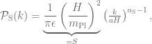
$\mathcal{P}_{\text{S}}(k) = \underbrace{\frac{1}{\pi \epsilon} \left(\frac{H}{m_{\text{Pl}}} \right)^2}_{=S} \left( \frac{k}{aH}\right)^{n_{\text{S}}-1},$

as well as the spectrum of the tensor perturbations (gravitational waves) in the form

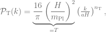
$\mathcal{P}_{\text{T}}(k) = \underbrace{\frac{16}{\pi} \left(\frac{H}{m_{\text{Pl}}} \right)^2}_{=T} \left( \frac{k}{aH}\right)^{n_{\text{T}}},$

where $H$ is a Hubble factor and $m_{\text{Pl}}\approx 1.22\cdot 10^{19}$ GeV is the Planck mass. Expressions for the scalar and tensor spectral indices are respectively

$n_{\text{S}} =1-4\epsilon$ and $n_{\text{T}} =-2\epsilon,$

where $\epsilon \ll 1$ is called a slow-roll parameter. Therefore, prediction from this so-called slow-roll inflation is that the scalar spectral index $n_{\text{S}}$ is almost equal to one but a little bit smaller (in jargon: red shifted). Let us confront this with the available CMB data. Recent results from the 7-years observations of the WMAP satellite [2] give

$n_{\text{S}} = 0.963 \pm 0.012.$

This is in full agreement with the prediction from the slow-roll inflation which supports the model. Moreover, the WMAP satellite measured also an amplitude of the scalar perturbations [2]

$S = 2.441^{+0.088}_{-0.092} \cdot 10^{-9}$

at the pivot scale $k_{0}=0.002 \ \text{Mpc}^{-1}$ . Based on the measurements of $S$ and $n_{\text{S}}$ one can compute the mass of inflation

$m \simeq m_{\text{Pl}} \frac{1}{4}\sqrt{3\pi S} (1-n_{\text{S}})=(1.4 \pm 0.5) \cdot 10^{-6} m_{\text{Pl}}.$

Therefore, the only parameter of the model can be recovered from the observational data. The crucial check of validity of this model would be given by measurements of the tensor power spectrum $\mathcal{P}_{\text{T}}$ . This spectrum can be however, detected only if the B-type polarisation of the CMB will be measured. While the B-type polarisation has not been detected yet, there are huge efforts in this direction. Experiments such as PLANCK [3], BICEP [4] or QUIET [5] are (partly) devoted to the search for the B-mode. The crucial parameterthat quantify the contribution of the gravitational waves is the so called tensor-to-scalar ratio $r$ . This is defined as a ratio of the tensor to scalar amplitude of perturbations at some given scale. Within the slow-roll inflationmodel, one can predict the value of $r$ , based on observation of the spectral index $n_{\text{s}}$ . Namely, a prediction of the slow-roll inflation model is the following

$r :=\frac{T}{S}=16\epsilon=4(1-n_{\text{S}})=0.15 \pm 0.05,$

where the value from WMAP-7 was applied. Moreover, based on WMAP-7 data, the tensor spectral index is predicted to be $n_{\text{T}}=\frac{n_{\text{S}}-1}{2}=-0.019 \pm 0.006$ . It is however unlikely to confront this quantity with observational data in the near future. Present observational constraints on the value of $r$ are

$r < 2.1 \ \text{at} \ 95 \% \ \text{C.L.} \ (\text{WMAP-7}),$

$r < 0.73 \ \text{at} \ 95 \% \ \text{C.L.} \ (\text{BICEP}),$

which come from the constraint on the amplitude of the B-type polarisation of the CMB. The predicted vale of $r$ is placed below the present observational limitations. However e.g. the PLANCK satellite (which is currently collecting the data) sensitivity reaches $r=0.05$ which is sufficient to detect the B-type polarisation as predicted by the slow-roll inflation. This would be a great support for the theory of inflation and the slow-roll model. However if, at this level of sensitivity, the B-type polarisation would not be detected, then the simple slow-rollinflaton would have rejected or required modifications. What will turn out to be a true? For the answer, we have to patiently wait till the end of 2012, when the first results from the PLANCK satellite will be released.

A. Linde, Lect. Notes Phys. 738, 1 (2008).
E. Komatsu et al., Submitted to Astrophs. J. Suppl. Ser., arXiv:1001.4538v1
[Planck Collaboration], “Planck: The scientific programme,” arXiv:astro-ph/0604069.
H. C. Chiang et al., “Measurement of CMB Polarization Power Spectra from Two Years of BICEP Data,” arXiv:0906.1181 [astro-ph.CO]
D. Samtleben and f. t. Q. Collaboration, “Measuring the Cosmic Microwave Background Radiation (CMBR) polarization with QUIET,” Nuovo Cim. 22B (2007) 1353 [arXiv:0802.2657 [astro-ph]].

Jakub Mielczarek

Theoretical physicist looking into the future

Month: December 2010

The origin of primordial perturbations